Language Modeling Foundations

To begin our discussion of what a language model is, we first have to formally define what a language is. The simplest structure we can start with is the idea of an alphabet, which is merely just a set of symbols denoted as \(\Sigma\). From our alphabet, we can build strings, which are finite sequences of symbols formed by concatenation. Since concatenation is associative, we can define a concatenative closure, often called the Kleene closure of an alphabet, denoted as \(\Sigma^*\). Intuitively, this is just the set of all finite strings generated from our alphabet. Since the Kleene closure also includes the empty string, it provides a nice monoid we can work with. We then define a language as a subset of \(\Sigma^*\).

Note on terminology: The terminology we use here is drawn from formal language theory. In practical settings, we can normally substitute “alphabet” with any building block we use for language, like a vocabulary that will be comprised of either words or tokens. A string will then be synonymous with what we call sentences, and our language will be a subset of all possible sentences.

We now have enough tools to define what a language model is. In natural language processing, we define a language model as a probability distribution over \(\Sigma^*\). There are two main types of language models, though only one is actually practical at the moment: we can either define one that is locally normalized (in which we define probabilities of strings through a sequence model) or globally normalized (which is energy based).

Globally Normalized Language Models

We will first talk about the less practical of the two models: globally normalized language models. A globally normalized language model is a model equipped with an energy function \(\hat{p}\), that maps values from \(\Sigma^*\) to the reals. Just as we commonly do in statistical learning theory, we define the unnormalized probability of a string \(y\) to be \(\text{exp}(-\hat{p}(y))\), and divide it by the normalization constant, \(Z = \sum_{y \in \Sigma^*}\text{exp}(-\hat{p}(y))\), to get the probability of generating that string. In other words:

At a first glance, this approach seems attractive since all we have to do is define an energy function to have our language model, which is often easier than setting a probability distribution. However, on a second glance, computing the normalization constant \(Z\) seems a bit unintuitive, as \(\Sigma^*\) contains infinitely many strings. Does it even converge? In addition, how would we sample?

Locally Normalized Language Models

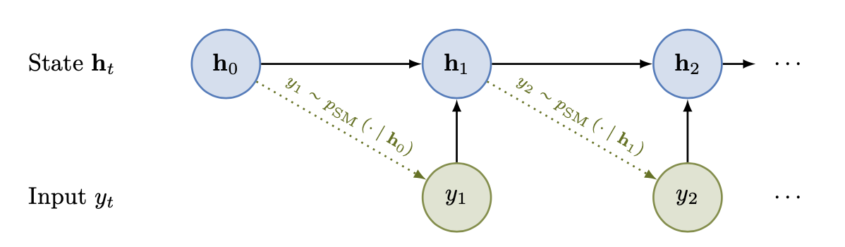
The inherent difficulty of computing the normalization constant motivates the definition of the locally normalized language model. Rather than directly defining a language model as a distribution over \(\Sigma^*\), we can break our problem down into pieces, by generating a string a symbol at a time. The idea is, for each possible context \(y \in \Sigma^*\), we define the probability distribution over the conditional \(y\). In other words, we define a sequence model \(p_{\text{SM}}\) such that

where

The probability of generating a string \(y\) is then

It’s tempting to think that we’re done. But we’re not. Notice how since probabilities are at most 1, the probability of generating a string decreases with its length. Thus, statements like “Upenn is in” are more likely to be sampled than “UPenn is in Philadelphia”. To get around this, we introduce the EOS (End of String) symbol into the distribution, so that \(p_{S\text{SM}}\) maps values from \(\overline{\Sigma} = \Sigma \cup \{\text{EOS}\}\) to the reals. We then have that

Count-Based N-gram Models

Having established the formal foundation for language models, let’s now explore one of the simplest practical implementations: count-based n-gram models. N-gram models make a strong Markov assumption that the probability of a word depends only on the n-1 preceding words. Formally, this gives us:

For instance, in a trigram model (n=3), we assume:

To estimate these probabilities, we use the maximum likelihood estimate (MLE) based on corpus counts:

where \(C(\cdot)\) denotes the count of occurrences in our training corpus.

Note on data sparsity: While n-gram models are conceptually simple, they suffer from data sparsity issues. As n increases, the number of possible n-grams grows exponentially, making it increasingly likely that valid n-grams will not appear in our training data, resulting in zero probabilities. This issue is particularly problematic because multiplying by zero in our chain rule formula would zero out the probability of the entire sequence.

To address this problem, we employ various smoothing techniques:

1. Laplace (Add-1) Smoothing: Add 1 to all counts: \(p_{\text{SM}}(y_l \mid y_{l-(n-1)}, \ldots, y_{l-1}) = \frac{C(y_{l-(n-1)}, \ldots, y_{l-1}, y_l) + 1}{C(y_{l-(n-1)}, \ldots, y_{l-1}) + |\Sigma|}\)

2. Add-k Smoothing: A generalization of Laplace smoothing where we add k (0 < k < 1) instead of 1.

3. Backoff Models: If an n-gram has zero count, we “back off” to the (n-1)-gram.

4. Interpolation: Combine probabilities from different order n-grams: \(p_{\text{interp}}(y_l \mid y_{l-(n-1)}, \ldots, y_{l-1}) = \lambda_1 p(y_l \mid y_{l-(n-1)}, \ldots, y_{l-1}) + \lambda_2 p(y_l \mid y_{l-(n-2)}, \ldots, y_{l-1}) + \ldots + \lambda_n p(y_l)\) where \(\sum_i \lambda_i = 1\) and \(\lambda_i \geq 0\).

5. Kneser-Ney Smoothing: A more sophisticated smoothing technique that considers the diversity of contexts in which a word appears, not just its frequency.

Despite their simplicity, n-gram models dominated the field of language modeling for decades. However, they have inherent limitations: they can only capture short-range dependencies due to the Markov assumption, and they suffer from the curse of dimensionality as n increases.

Representation-Based Models

The limitations of n-gram models motivate the development of representation-based approaches, which learn continuous vector representations (embeddings) of words and contexts.

Word Embeddings

Word embeddings map words from a discrete space (the vocabulary) to a continuous vector space \(\mathbb{R}^d\), where semantically similar words are positioned closer together. This addresses two fundamental issues with n-gram models:

1. They capture semantic relationships between words, enabling better generalization.
2. They provide a more compact representation, mitigating the curse of dimensionality.

1. Count-based methods: Such as Latent Semantic Analysis (LSA), which applies singular value decomposition to word-context co-occurrence matrices.

2. Prediction-based methods: Like Word2Vec (Skip-gram and CBOW) and GloVe, which learn embeddings by predicting words given their contexts or vice versa.

For instance, in the Skip-gram model, we maximize:

where c is the context window size, and

Here, \(v_w\) represents the vector embedding of word w.

Recurrent Neural Networks (RNNs)

Embeddings provide a powerful way to represent individual words, but language modeling requires capturing sequential dependencies. Recurrent Neural Networks (RNNs) address this by maintaining a hidden state that evolves as they process a sequence, enabling them to capture long-range dependencies beyond the fixed context window of n-gram models.

Intuition for RNNs

The key intuition behind RNNs is that they mimic how humans process language sequentially while maintaining context. When we read or hear a sentence, we don’t start from scratch with each new word; instead, we update our understanding based on previous words. RNNs formalize this by maintaining a hidden state that acts as a “memory” of what has been seen so far.

Consider the sentence “The cat sat on the mat.” As we process each word:

1. “The”: Initialize our context (this is a determiner, likely to be followed by a noun).
2. “cat”: Update our context (now we know the subject is a cat).
3. “sat”: Update again (now we understand the action). And so on.

This sequential processing with memory enables RNNs to model complex language phenomena like agreement, ambiguity resolution, and even limited forms of reasoning.

Technical Details of Simple RNNs (Elman Networks)

Formally, an Elman RNN processes a sequence \(y_1, y_2, \ldots, y_L\) as follows:

1. Each word \(y_t\) is first converted to its embedding representation \(e_t = E_{y_t}\).

2. The network computes a hidden state \(h_t\) based on the current input and the previous hidden state:

   \[h_t = \tanh(W_h h_{t-1} + W_x e_t + b_h)\]

   where \(W_h \in \mathbb{R}^{d_h \times d_h}\) is the hidden-to-hidden weight matrix, \(W_x \in \mathbb{R}^{d_h \times d}\) is the input-to-hidden weight matrix, and \(b_h \in \mathbb{R}^{d_h}\) is a bias term. The initial hidden state \(h_0\) is typically set to a vector of zeros.

3. The output layer then converts the hidden state into a probability distribution over the vocabulary for the next word:

   \[o_t = W_o h_t + b_o\] \[p(y_{t+1} | y_{\leq t}) = \text{softmax}(o_t)\]

   where $$W_o \in \mathbb{R}^{

   \Sigma

   \times d_h}\(is the output weight matrix and\)b_o \in \mathbb{R}^{

   \Sigma

   }$$ is the output bias.

Specifically, the softmax function converts the output logits into a proper probability distribution:

where \(o_{t,w}\) is the component of the output vector corresponding to word w.

Training RNNs

RNNs are trained using the maximum likelihood principle, which for language modeling translates to minimizing the negative log-likelihood of the training data:

This is often referred to as minimizing the cross-entropy loss. The optimization is done using backpropagation through time (BPTT), which is a variant of the standard backpropagation algorithm adapted for sequential models. In BPTT, we unroll the RNN for a fixed number of steps and then apply backpropagation to compute gradients.

Challenges with Simple RNNs

While simple RNNs (Elman networks) represent a significant improvement over n-gram models, they still face challenges:

1. Vanishing and exploding gradients: During training with BPTT, gradients can either vanish or explode as they are propagated back through time, making it difficult to learn long-range dependencies.

2. Limited memory capacity: The fixed-size hidden state can struggle to retain information over very long sequences.

These challenges led to the development of more sophisticated architectures like Long Short-Term Memory (LSTM) networks and Gated Recurrent Units (GRUs), which incorporate gating mechanisms to better control information flow and mitigate the vanishing gradient problem.

Conclusion

We have covered the foundations of language modeling, from formal definitions to practical implementations. We started with count-based n-gram models, which make strong Markov assumptions but suffer from data sparsity and limited context. We then moved to representation-based approaches, discussing word embeddings that capture semantic relationships and RNNs that model sequential dependencies.

This progression reflects the historical development of language modeling, with each approach addressing limitations of its predecessors. Modern language models build upon these foundations, incorporating attention mechanisms, transformers, and pre-training on massive corpora to achieve unprecedented performance across a wide range of natural language processing tasks.

As language modeling continues to evolve, understanding these foundational concepts remains crucial for developing intuition about how these models work and their inherent strengths and limitations.